Unit 9 (May)
Simplifying Rational Expressions: A Rational expression is an expression that is a fraction. We have been dealing with these expressions for the last 2 years, however, in Algebra when we refer to Rational Expressions we are generally referring to ones that are a little more difficult.
See the video below:
See the video below:
Solving Proportions with Quadratic terms: There are a few different ways to solve a proportions with quadratic expressions (I review them in the video below), but chances are that cross multiplying will be easiest. Recall that cross multiplying works based on the idea if two fractions are equal, then their cross products must also be equal.
Adding, subtracting, multiplying, and dividing rational expressions: A rational expression is simply a fancy way of say 'fractional' expressions. We have already worked on how to simplify rational expressions with one term when we simplified exponents (for example: simplify 2xy / 4x).
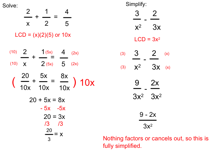
Remember, to add or subtract fractions we first need a common denominator, and then we add or subtract the numerators. Lastly, we simplify the sum or difference (for example, if you add two fractions and get 2/4, you would simplify this to 1/2).
To get the common denominator, we follow the same rules that we used when find the LCD in 4th grade.
Below is one solving equation example, and one simplifying example:
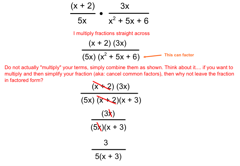
Below is an example of multiplying expressions. Please note that I am not showing you how to "solve" an equation involving multiplying polynomial fractions, just how to multiply and then fully simplify your product.
Also, note that you divide fractions by multiplying by the reciprocal. I am not going to provide an example of this :)
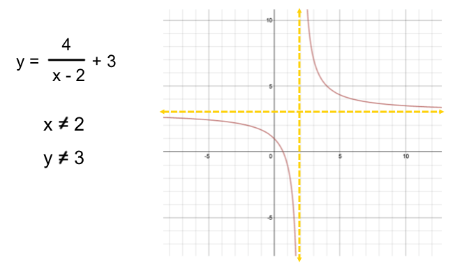
Graphing rational equation in Function Form: This is where rational expressions get interesting......graphing. There are two types of rational equations we will be graphing. Equations in standard form, and equations in factored form. Equations in standard form follow the following formula:
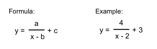
Looking at the example above, think of values that you cannot have for x. Since you have a fraction, you know that the denominator cannot be 0. Knowing this, that means x cannot be 2 (because 2-2 =0). Therefore, the graph will get closer and closer to x=2 but will never touch it. Therefore, the graph will have a vertical boundary (called an asymptote) at x =2. Why vertical? Because x = 2 is a vertical line.
What about horizontal boundaries (asymptotes)? Well, if x could be 2, then y = 4/0 + 3. That means y = 0 + 3 or 3. So, since x cannot equal 2, that means y will never equal 3. Therefore there is a horizontal asymptote at y = 3.
The 2 asymptotes will form a 'centerpoint' when x = 2 and y = 3, so the point (2, 3). While the graph will appear to get closer to each line without touching them. See the example below:
If we take the above standard form equation and simplify the right side of the equation together, we get this:
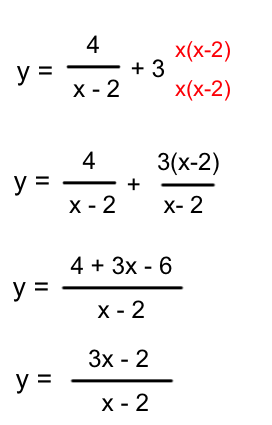
In this new form (called factored form) x cannot be 2 still, so we see the vertical asymptote. However, we cannot readily see the vertical asymptote. The standard form equation is best used when finding both asymptotes (if any). However, this factored form has its own benefits.
Using factored form, you will be able to easily find asymptotes, holes, x-intercepts, and y-intercepts.
Using factored form, you will be able to easily find asymptotes, holes, x-intercepts, and y-intercepts.
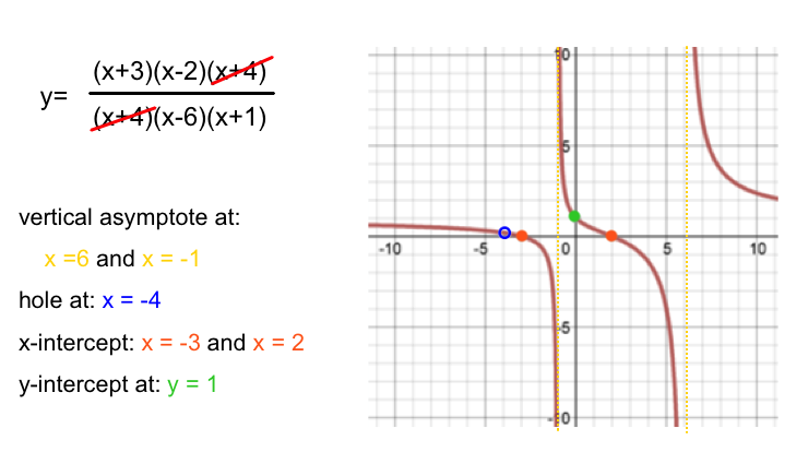
Graphing Rational Equations in Factored form: See the factored rational equation below:
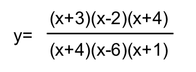
In this equation, you may notice that (x+4) appears in both the numerator and denominator. This means that (x+4) will cancel out, so the equation turns into:
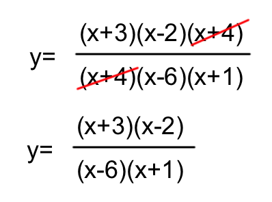
In this new simplified equation, x cannot equal 6 or -1. This means you will have vertical asymptotes at 6 and -1. Similarly, (x+4) canceled out earlier. You cannot simply forget that (x+4) was a part of the original equation, even though it canceled out. In the initial equation x could not be 4 too, therefore you have something 'missing' when x=4. However, it isn't exactly an asymptote because x could certainly be equal to 4 in the new equation. Therefore, you must make a note of what x could not be initially (4) and draw a 'hole' at that point on the graph. The 'hole' is literally an open point or circle (a hole) at x=4. It represents a point on a graph that you cannot have.
Next we have the x-intercepts. An x-intercept occurs when y=0. In order to get y=0, the numerator must also equal 0 (because 0 divided by anything will equal 0). So in the numerator above, x cannot be equal to -3 or 2. Therefore, when y=0, x=-3 or x=2. These are your x-intercepts.
Lastly, the y-intercepts. Slightly more involved (but not really). The y-intercept occurs when x = 0. So you can literally plug in 0 for x and find out what y equals. y = (3)(-2) / (-6)(1) or y = -6 / -6 = 1. Therefore, when x=0, y = 1. This is your y-intercept.
Now you are ready to graph these boundaries on the graph.
Note: You are not actually graphing the equations, just the boundary information. You will learn in higher level math classes how to graph the actual equation. For now, I will ask for you to find these parts, or I will give you a graph and ask you to write a possible equation that would make it.You will not have to know 'how' to graph the equation itself, just how to find the parts above, and recognize how they relate to the equation.
Long division of polynomials: Recall the different ways to show the division of two numbers:
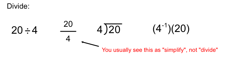
In each scenario above, I can easily attain an answer / simplified value of 5 (with no remainder). We can also attempt each method with numbers that do not go easily into one another:
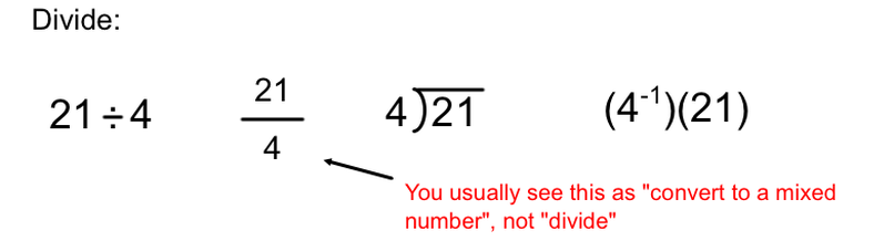
In each case, we would divide and get 5.25 or 5 and a remainder of 1/4. Since we can do these "skills" easily with numbers, we can therefore perform the same "skills" shown above with variables and polynomial expressions too. Exciting!!!....
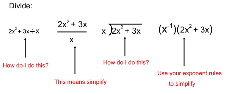
Since we have already covered the second and fourth skills above, we will focus on using long division (the division symbol seen in the first method typically means or encourages you to use a calculator....obviously we cannot do this with variables).
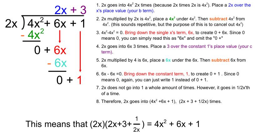
Refresh your memory of long division below, then apply this to the polynomial example:
Refresh your memory of long division below, then apply this to the polynomial example:
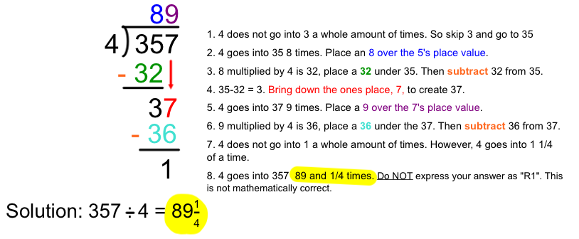
Now, see how these steps apply to long division of polynomials: