Unit 3 (December)
Solving Systems of Equations by Graphing: A system of equation is simply a group of equation with like-variables (most equations are written in standard form for "ease" of solving, but they can be written in any form). When you 'solve' a system, you are looking for the common values that you can plug in for each variable. For example, consider the system:
x + y = 5
x - y = 1
Try to think of an x and y value that would work for the first equation, 1 and 4, 2 and 3, 3 and 2, 2.5 and 2.5, -8 and 13.... There are an infinite combinations of x and y values. The same predicament exists for the second equation (infinite combinations). However, to solve this as a "system" you are looking for that one single combination of x and y values that works in both equations. In this case, x=3 and y = 2 is the only combination of numbers that works. Therefore, x=3, y=2 is the solution. We can also say this solution as the point (3, 2).
Therefore, graphically you are looking for the x and y values on a graph where the two equations are equal to one another. Or in other words, their point of intersection.
For example:
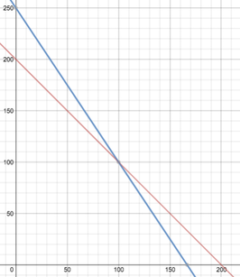
Suppose you are selling tickets for a school play to adults and kids. The number of tickets you sell total 200, and you make $500. If adult tickets cost $3 each, and kids' tickets are $2 each, how many of each ticket did you sell?
To begin, you can create the following equations:
a + k = 200 <----------- This equation represents the "quantity" of each ticket sold
3a + 2k = 500 <--------- This equation represents the "cost" of each ticket sold
In each case, 'a' stands for the number of adult tickets and 'k' stands for the number of kids' tickets. Therefore, a + k = 200 total tickets, and $3.00 times the number of adult tickets sold + $2.00 times the number of kids' tickets sold = the total money made.
When you graph this system (at right), the point where they intersect is the point for (a,k) that satisfies both equations. In this case, (100,100). Therefore, you sold 100 adult and 100 kids' tickets.
Solving systems of equations using Substitution: The substitution method involves solving one of your equation for a single variable and plugging it into the other equation.
Solving using substitution
Solving using substitution video
For example, take the scenario above....Suppose you are selling tickets for a school play to adults and kids. The number of tickets you sell total 200, and you make $500. If adult tickets cost $3 each, and kids' tickets are $2 each, how many of each ticket did you sell?
These are your equations from above:
a + k = 200
3a + 2k = 500
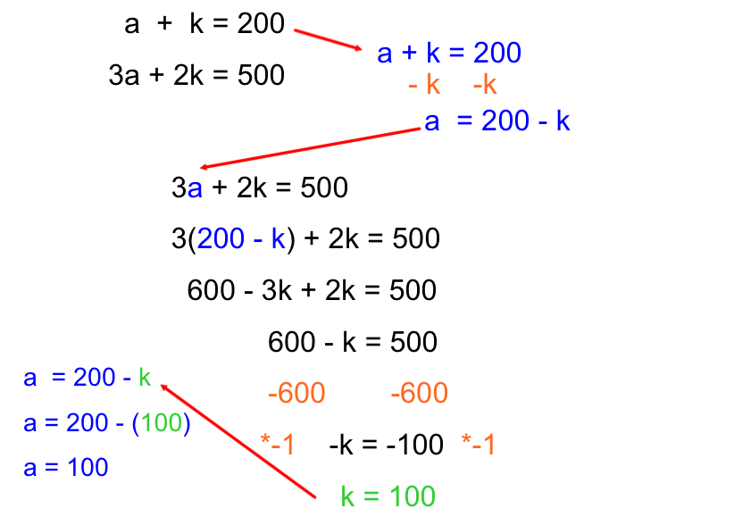
If the number of adult tickets + kid tickets total 200, then you can find the number of adult tickets by subtracting the kid tickets from 200. Right?
Algebraically, if a + k = 200, then a = 200 - k.
Therefore, if a = 200 - k then "200 - k" is interchangeable with "a" (they equal each other after all).
So instead of writing 3a + 2k = 500, you can write this as 3(200 - k) + 2k = 500. Why would you do this? Because now you only have one variable, k, to solve for. You can certainly solve this equation to determine the number of kid tickets sold, and use that number to determine the number of adult tickets sold. See this example's algebraic work shown below:
x + y = 5
x - y = 1
Try to think of an x and y value that would work for the first equation, 1 and 4, 2 and 3, 3 and 2, 2.5 and 2.5, -8 and 13.... There are an infinite combinations of x and y values. The same predicament exists for the second equation (infinite combinations). However, to solve this as a "system" you are looking for that one single combination of x and y values that works in both equations. In this case, x=3 and y = 2 is the only combination of numbers that works. Therefore, x=3, y=2 is the solution. We can also say this solution as the point (3, 2).
Therefore, graphically you are looking for the x and y values on a graph where the two equations are equal to one another. Or in other words, their point of intersection.
For example:
Suppose you are selling tickets for a school play to adults and kids. The number of tickets you sell total 200, and you make $500. If adult tickets cost $3 each, and kids' tickets are $2 each, how many of each ticket did you sell?
To begin, you can create the following equations:
a + k = 200 <----------- This equation represents the "quantity" of each ticket sold
3a + 2k = 500 <--------- This equation represents the "cost" of each ticket sold
In each case, 'a' stands for the number of adult tickets and 'k' stands for the number of kids' tickets. Therefore, a + k = 200 total tickets, and $3.00 times the number of adult tickets sold + $2.00 times the number of kids' tickets sold = the total money made.
When you graph this system (at right), the point where they intersect is the point for (a,k) that satisfies both equations. In this case, (100,100). Therefore, you sold 100 adult and 100 kids' tickets.
Solving systems of equations using Substitution: The substitution method involves solving one of your equation for a single variable and plugging it into the other equation.
Solving using substitution
Solving using substitution video
For example, take the scenario above....Suppose you are selling tickets for a school play to adults and kids. The number of tickets you sell total 200, and you make $500. If adult tickets cost $3 each, and kids' tickets are $2 each, how many of each ticket did you sell?
These are your equations from above:
a + k = 200
3a + 2k = 500
If the number of adult tickets + kid tickets total 200, then you can find the number of adult tickets by subtracting the kid tickets from 200. Right?
Algebraically, if a + k = 200, then a = 200 - k.
Therefore, if a = 200 - k then "200 - k" is interchangeable with "a" (they equal each other after all).
So instead of writing 3a + 2k = 500, you can write this as 3(200 - k) + 2k = 500. Why would you do this? Because now you only have one variable, k, to solve for. You can certainly solve this equation to determine the number of kid tickets sold, and use that number to determine the number of adult tickets sold. See this example's algebraic work shown below:
Solving systems of equations using elimination: The elimination method involves 'combining' the two equations in such a way that one variable cancels out or is 'eliminated'. Thus allowing you to solve for the remaining variable.
Example 1:
2x + 3y = 6
-2x + 4y = 8
When combined (or added), these system above turns into 7y = 14. Therefore y = 2. You can now plug this into either equation and solve for x.
Example 2:
2x + 5y = 12
4x + 3y = 10
When combined, no variable will 'eliminate' above. However, you can use the knowledge that you can multiply entire equations (for example, y = 6 also means 2y = 12, or 2y + 1 =13, etc etc).
By multiplying the top equation by -2, your system becomes:
- 4x - 10y = -24
4x + 3y = 10
Now you can combine equations to eliminate x and solve for y.
Solving using elimination Video with examples
Solving "special" systems of equations: To this point, we have dealt with systems that have one nice 'easy' solution, but what if our system did not have a solution? What if our system had more than one solution? What does this mean?
You may want to review what it means when you arrive at "no solution" or "all real numbers" (infinite) solutions. Go to the intro unit tab above, and scroll down to the third concept. Since you should already know what these concepts mean I am going to focus more on the graphic meanings of infinite and no solution below
One solution: A system has one solution when their equations have one single point of intersection on a graph. There is only one x and y value that makes the two equations equal to one another.
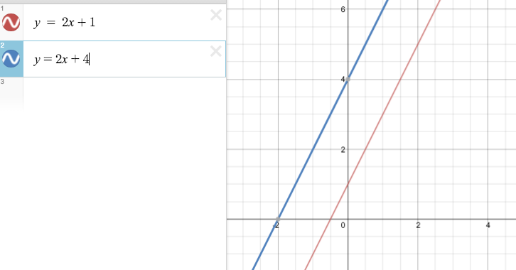
No solution: A system has no solution when their equations have no points of intersection on a graph. There are no x and y values that makes the two equations equal to one another. Graphically, this means the equations are parallel to each other. Algebraically, this means that if we were to set the equations equal to one another and solve for x there would be no solution.
Infinite solutions: A system an infinite number of solutions when their equations have one single point of intersection on a graph. There is only one x and y value that makes the two equations equal to one another. Graphically, this means that the two equations are exactly the same and therefore lie on top of one another. Algebraically, this means that if we were to set the two equations equal to one another that they would have 'all real numbers' as a solution.
Choosing the best method for solving a system: Choosing the best method is rather simple, but it takes some math logic and reasoning skills. Why bother? Because one day you may take a midterm (wink wink), placement test, SBAC test, CAPT, SAT, etc..... On these exams you are never told "Solve this system using substitution" or "Solve this system using elimination". You are simply told "Solve this system". Therefore, you need to be able to accurately and choose which method is easiest and most efficient. The last thing you want to do is spend 15 minutes on a problem that should have taken 2 because you missed an obvious "hint" that you should use one method over another:
One thing to remember: ALL METHODS will work with ANY system. However, we are simply going to talk about which method is preferred. Likewise, you may have more than one "preferred method" for a given system, and that is fine. As long as you realize that, and you don't choose the one method that was more time consuming.
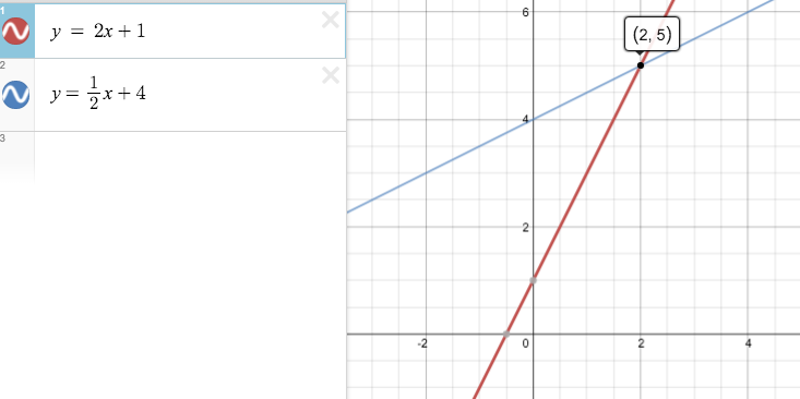
Substitution: Recall that the substitution method involves solving one of your equation for a single variable and plugging it into the other equation. This method is best used when you have a variable that is already isolated, or has a coefficient of one. For example:
x + 3y = 5 y =2x + 1 2x - 6y = 10 y = 2
4x - 7y = 10 4x + 5y = 7 5x + y = 1 3x + 8y = 9
Graphing: Recall that when you solve graphically you are quite literally graphing the equations and finding the point of intersection. Therefore, solving graphically might be easier when you have a system where both equations are written in slope-intercept form. Similarly, some real life systems may have annoying fractions and decimals that provide you with just as annoying fraction/decimal solutions. So for the most part, when you have a seriously crazy system you have to ask yourself "is this easier to solve using substitution or elimination? Or is it just easier to throw it onto desmos?". This sounds like a no brainer, but if you have access to a graphing calculator of some kind why not use it? This is obviously assuming you are allowed to use a graphing calculator. For example:
Seriously? why bother?
y = 2x + 5 .243x + 6.501y = -23.4 2/3x - 1.6y = 13/7
y = 3x - 1 . 777x - 1.2y = 17.2341 .24x + 9/7y = -12/13
Elimination: Recall that the elimination method involves "combining with the purpose of eliminating". This is your "bulldozer" of systems methods because it involves the most work. We would prefer to use the elimination method when we see terms that would easily cancel out when combined (see the first system below), or when we can perform a simple operation to enable us to easily combine and cancel (see the second system below). Similarly, we would use elimination when we can't use graphing, or when substitution doesn't make sense. Basically, if a system has an isolated variable we would use substitution, when both equations are easily "graphable" we would use graphing, and when all else fails we would simply use elimination. For example:
3x + 2y = 5 2x - 5y = 1 2x - 4y = -12
4x - 2y = 10 9x + 10y = 8 7x + 9y = 3
cancel the y's double your top equation first Be like Nike, and just do it!!
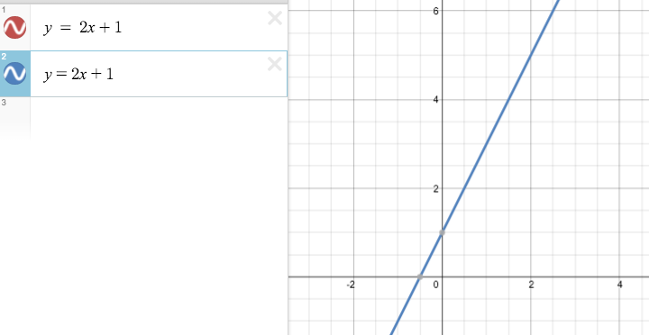
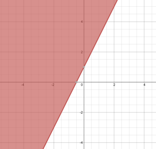
Graphing two-variable inequalities: Graphing inequalities is very simple, provided that you recall how to graph a normal equation in slope-intercept form. If you wanted to graph y = 2x + 1 your y-intercept will be at 1, and you will have a slope of 2. Graphing y > 2x + 1 means that your y value could be equal to 2x + 1, but it could also be more than. Therefore, we would still graph the line y = 2x + 1, but we would also 'draw' in all values greater than this line. That is, we shade in the entire area above the line. The trick here is that if you put your pencil directly on the line, shade above this point. Since y "could be" equal to 2x + 1, we are also correct in leaving a solid line at y = 2x + 1.
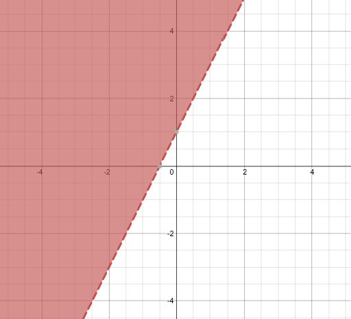
But what about > or < ? These are just as simple, but there is one extra step. If you were graphing y > 2x + 1, you still graph the line y = 2x + 1 and shade above. However, you want to indicate that y is ONLY greater than (or less than for that matter) we use a dotted line (recall that when graphing x > 4 on a number line we use a hollow dot. A dotted line is a "hollow line").
See the examples below:
y > 2x + 1
y > 2x + 1
y > 2x + 1
y > 2x + 1
Graphing systems of inequalities: When graphing a system of inequalities, the solution becomes a little more "interesting". For example, consider the system with inequalities A and B:
A: y > 1/2x + 2
B: y < 3x + 1
The solution set to this system includes all points more than A, but less than or equal to B.
A: y > 1/2x + 2
B: y < 3x + 1
The solution set to this system includes all points more than A, but less than or equal to B.
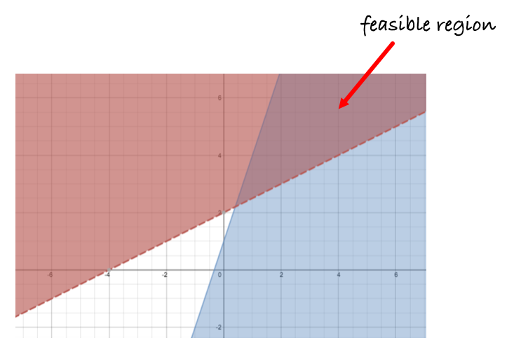
The solution to the system above (shaded in purple) is known as the "feasible region". A feasible region is the area where points reside that could be a possible solution to a system.
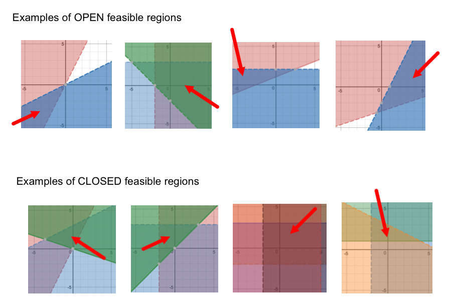
Open versus Closed solution: An "open" feasible region is a solution that is unbounded on one or more sides, while a "closed" feasible region is a solution that has boundaries (or constraints) on all sides. For example, see below:
Linear Programming: Linear programming is a mathematical term for using a system of inequalities to find the optimal or best point to use out of an infinite number of possible solutions. Typically, there is a large quantity of data and information in a linear programming problem, therefore, the underlying skill that linear programming requires is organization and creative problem-solving. By this I mean creating a feasible step by step method to approach and attack a problem of this magnitude. To further explain this, watch the video below:
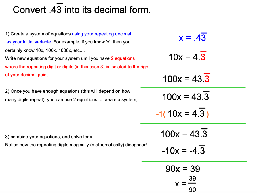
Converting repeating decimals to fractions:
Last year we learned how to take a fraction, like 7/8, and use long division or proportions to convert it into its decimal form. Now, we already know how to convert terminating decimals into fractions using our knowledge of place value. However, we have not been able to convert repeating decimals into their fraction form (unless they are common knowledge, like .3333333....). Using our knowledge of systems we can do just that, convert any repeating decimal into its fraction form.
Help website with examples
The Midterm exam will cover September through December content.
For copies of study guides and materials handed out in class, click here: Midterm review packet
Content below this title will not appear on the Midterm.
Unit 4 (January)
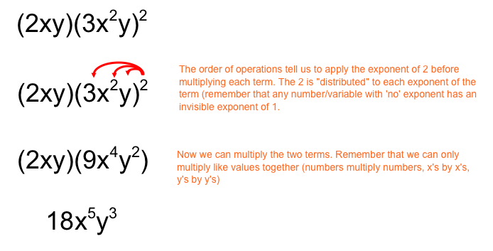
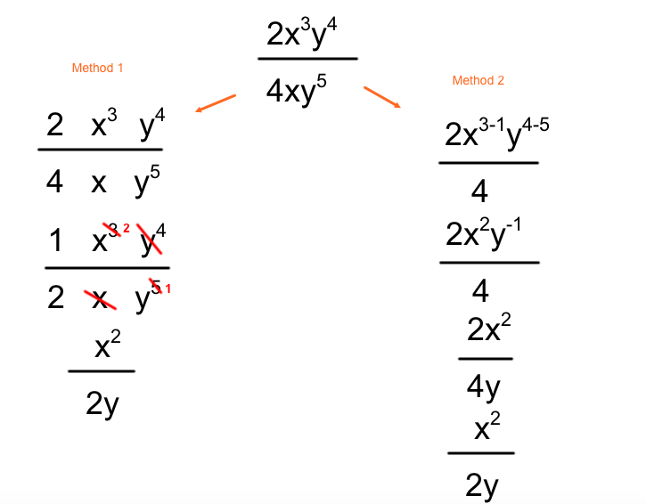
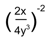
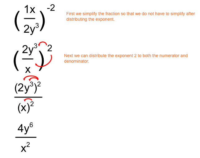
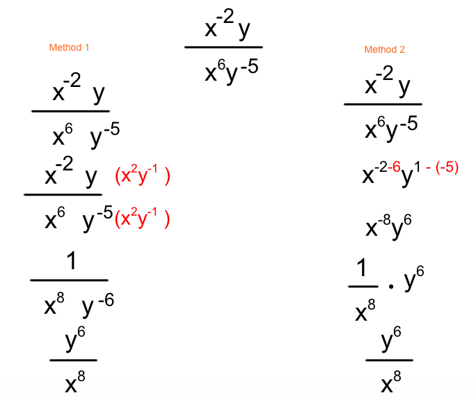
Operations with exponents - Exponents can be very tricky because there are so many different rules to use and remember. However, there is no single way to approach an exponent problem, so as long as your steps are mathematically correct you can follow any path you choose. I will provide a few examples below. Please note that there may be more possible methods than those shown below:
Basic multiplication rules
Negative and 0 exponent rules
Watch the first 9 videos (on the left) for examples on everything we will do with exponents
The 3 videos linked below will show you some of the basics that we will cover this month:
Basic multiplication rules
Negative and 0 exponent rules
Watch the first 9 videos (on the left) for examples on everything we will do with exponents
The 3 videos linked below will show you some of the basics that we will cover this month:
Example 1:
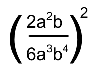
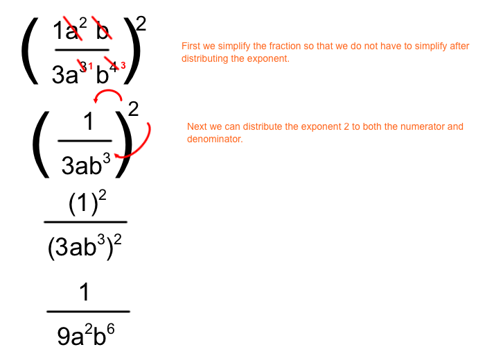
Example 2:
Example 3:
Example 4:
Example 5:
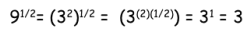
Rational exponents: These are exponents that happen to be fractions, like 9^(3/2). Using your knowledge of exponent rules, you know that (a^m)^n = a^(mn). Also, using your knowledge of fractions you know that fractions multiply straight across. See the example at the right to see how this plays out.
We will revisit rational exponents in another unit, there is more to them than meets the eye..... :)
Rational exponent examples
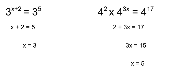
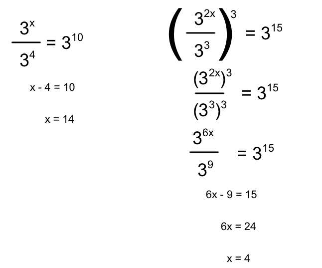
Solving for exponents: This is not so much a "concept" as an idea that you can use your rules to find missing numbers in exponents. Think about it as solving an equation where the variables occur in the exponents. See the examples below:
Graphing exponential functions: Exponential functions are equations in the form:
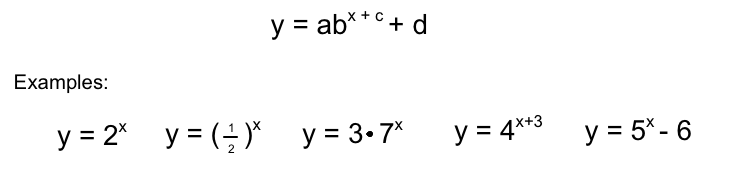
Note that this is not an "official" formula, but more of a general guideline. The one thing that remains common between each example above is the fact that "x" is the exponent to a numerical base. In general, we will focus more on the first two example above, but you should be aware that as long as 'x' remains my exponent, I can write an "exponential function" similar to either of the examples above.
In Algebra 1, we will focus our attention on exponential functions where your base 'b' is an integer, and when b is a fraction above 0 but less than 1.
Observe the graphed examples below:
In Algebra 1, we will focus our attention on exponential functions where your base 'b' is an integer, and when b is a fraction above 0 but less than 1.
Observe the graphed examples below:
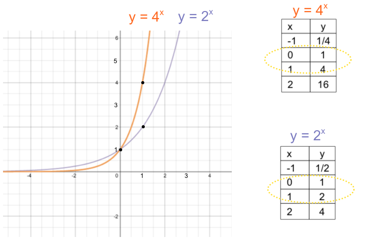
Notice how in both cases that when your exponent is "1" (x=1) your y-value is simply your base's value. This is because any number to the exponent of one will be itself. Similarly, notice that when the exponent is 0 both graphs have a y-value of 1. This is because any number to the exponent of 0 is equal to 1. With this knowledge, we can determine the equation of almost any exponential function by simply knowing the points (0, 1) and (1,y).
For example, the exponential equation that passes through the points (0,1) and (1 , 7) is y = 7^x.
*In this example, knowing the point (0,1) is not terribly important to "creating the equation", however, we need to know that this point exists to confirm that the points are indeed increasing exponentially.
Exponential growth and decay: Something is growing exponentially when its value continues to multiply, or compound, by itself over and over again. By comparison, exponentially decaying means the value is being divided by itself over and over again (or multiplied by the fraction equivalent of dividing).
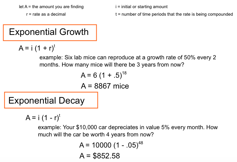

Some real life examples of exponential growth and decay:
Growth Decay
- A bacteria cell population doubles every minute for 10 hours - A car depreciates in value by 12% every year
- A bank account earns 2% interest every month for 3 years - A tin can decomposes a third of its mass
- A population of mice can quadruple in size every 13 days every 95 years
- A radioactive element has a half life of 400 years
Key words for this lesson:
compound - To multiply over and over by the same number
depreciate- To go down in value (to "appreciate" means something goes up in value. So when you "appreciate" my help, that means my help is being valued) :)
half-life- The time it takes for an element (radioactive) to decay/decompose to be half (50%) of its initial mass
compounded daily- multiplied daily or 365 times a year
compounded annually- multiplied yearly or once every year
compounded biannually- multiplied every 6 months or twice a year
compounded quarterly- multiplied every 3 months or 4 times a year
Interest vs. Annual Interest
When calculating the interest rate to use in our formula, there is a big difference between interest and "annual interest". Take the following investment opportunity for example:
You are investing $3000 for 3 years into one of the following accounts:
A- 2% interest compounded quarterly: This means that you will earn 2% interest 4 times per year, 2%, 2%, 2%, and 2%.
i = 3000, r = 2% or .02, t = 12
B- 2% annual interest compounded quarterly: This means that you will earn 2% interest TOTAL across four quarters, .5%, .5%, .5%, and .5%
i = 3000, r = .5% or .005, t = 12
Geometric Sequences: Recall that an arithmetic sequence is a pattern of numbers in which you are adding the same common number between each value (for example, 3, 5, 7, 9...). A geometric sequence is a pattern in which you are multiplying by a common number (note, this number can be a whole number, fraction, positive, or negative)
Some examples are below:
5, 10, 20, 40, 80..... .5, .25, .125, .0625..... 1, 1, 1, 1, ..... 10, 15, 17.5, 26.25....... 3, 12, 48, 192.....
To create an explicit equation to model each sequence we must know two things. First, the starting point, and second, the common ratio between each value (this is simply the number that we are multiplying by to move from one value to the next).
Take the first sequence above for example. Starting at 5, you may notice that we are multiplying by 2 with each successive value. If 5 is our first value, we multiply once by 2 to get the second value, twice by 2 to get the third value, three times by 2 to get the fourth value, and so on.... Algebraically, I want to show that I am taking 5, and then multiplying by 2 a certain number of times. However, notice that to get each term we multiply by two one less time than the place value we are searching for (to get the 5th value, we multiply 4 times). So our equation will look something like this:
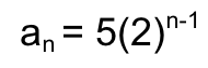
The formula to create any geometric sequence is as follows:
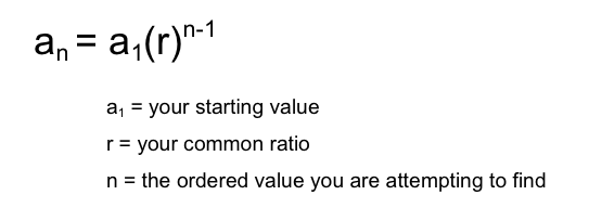
For example, suppose we wanted to find the 6th number in the previous pattern. I would input 6 for n, and evaluate 5(2)^5 = 160.
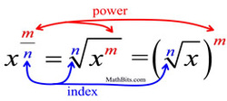
Rational Exponents: We will be going over "rules of radicals" in a later unit, however, for now we will cover exponents that are fractions (rational exponents). The rule for rational exponents is at right
Example:
Rational Exponents: We will be going over "rules of radicals" in a later unit, however, for now we will cover exponents that are fractions (rational exponents). The rule for rational exponents is at right
Example:
Pythagorean Theorem: The pythagorean theorem is a formula that relates all of the side lengths of a right triangle. Why are we going over this now? Because it involves squaring and square roots and fits in well with the current concepts. The video below shows us one way to derive, or create, this formula.
Example:
Diagonal of a rectangular prism: Use the following image as a guide for your diagonal word problems.
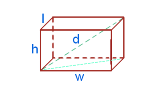
Also, the video below provides you with an example word problem:
Distance formula: Using the pythagorean theorem, we can find the distance between any two given points. Rather than explain this "in depth" formula, watch this video:
Midpoint: Using your logic and reasoning abilities, we discovered how to find the midpoint between two random points. If given two points, the 'midpoint' is considered the point halfway between each point. We expressed this two different ways.
1) Using Slope: If the slope between one point and another is 4/5, then the midpoint must be proportional but halfway between. Therefore, rather perform a rise/run of 4/5, you would rise 2 and run 2.5.
2) Using Mean: If given two numbers, the value between them must be their mean (or median for that matter). Therefore, if given two coordinate points the midpoint between them must be the mean of the x values and the mean of the y-value.
